Biology, read from a geneticist's source

Co-authored by Claude · Version 1.0.0, changed in rev 145

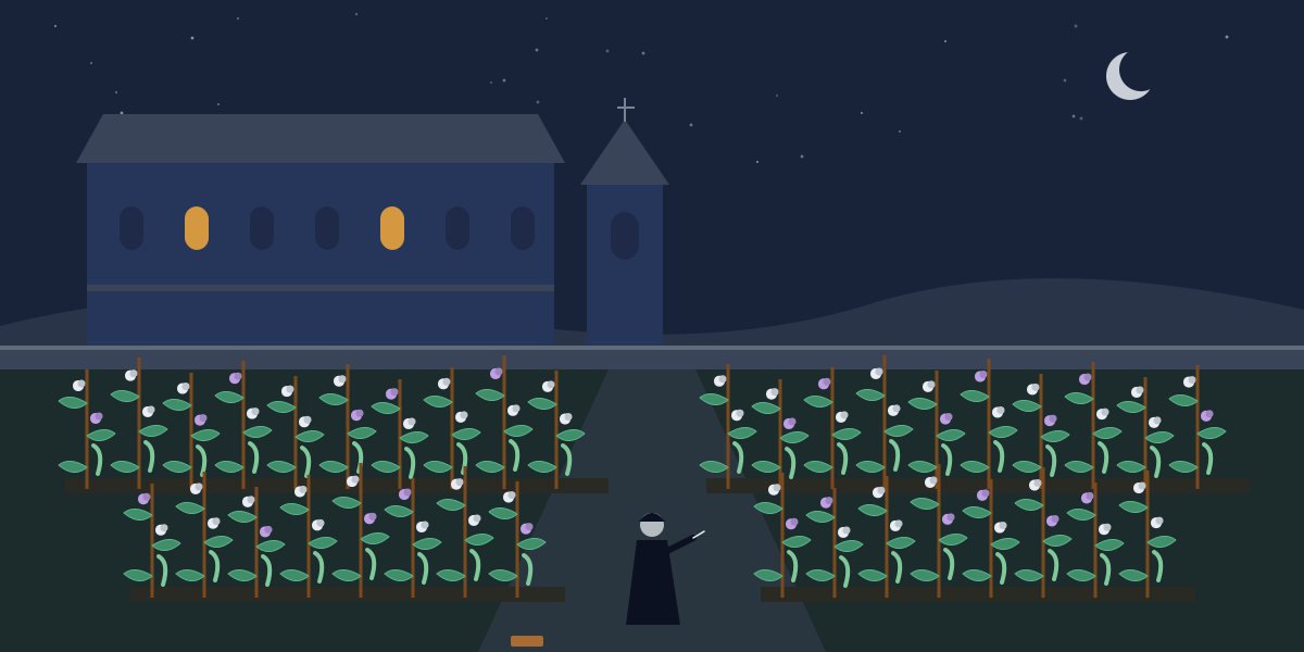
On 8 February and 8 March 1865 Gregor Mendel read a paper to the natural history society of Brünn, and in 1866 the society published it as Versuche über Pflanzenhybriden. Between 1856 and 1863 he had grown some 28,000 plants, most of them peas, and crossed varieties that differed in one trait, round seeds against wrinkled, yellow against green. The first generation all showed one form, and the second showed both, in a ratio of three to one; crossing plants that differed in two traits gave four kinds of offspring in the ratio 9 : 3 : 3 : 1. The paper was read by few and understood by fewer until 1900, when Hugo de Vries and Carl Correns, and by some accounts Erich von Tschermak, independently came to the same results. William Bateson suggested a name for the new science in a letter of 1905, and proposed it in public at a conference in London the next year: "I suggest for the consideration of this Congress the term Genetics."

The biology library for DKE, the Deterministic Knowledge Engine, writes some of that science down in DKE Python, and this essay teaches the biology by reading it. You record two kinds of fact. A metabolic network is its compounds and reactions, and the library's rules conclude what the network can make from what it is fed. A pedigree is its people and their parents, and the rules conclude each person's ancestors, a child of related parents, the carriers a mode of inheritance requires, and anyone the mode cannot explain. Each answer names the facts it rests on, and correcting a fact withdraws the answers it supported. The second half of the library calculates: crosses and the test of their counts, the genetic code, the growth of populations, genetic drift, and a ring of genes that switch one another off. Every program below runs as shown once the library's source file has been compiled into a store, and every output is copied from a run.

1. A cross

A gene comes in forms, its alleles, and a plant carries two copies of each gene, one from each parent. Write a genotype two letters a gene, the capital for the dominant allele, and a parent's gametes are every way of taking one allele of each gene. cross() pairs every gamete of one parent with every gamete of the other, and phenotypes() reads each offspring by what it shows, which is the dominant form wherever there is one dominant allele:

def phenotypes(a: string, b: string) -> dict<string, int>:
    for z in genotypes:
        for g in range(len(z) // 2):
            p = p + z[2 * g]

Here are a cross of two plants that each carry one copy of each allele, and the same for two genes:

import biology

print(biology.gametes("AaBb"))
print(biology.cross("Aa", "Aa"), biology.phenotypes("Aa", "Aa"))
print(biology.phenotypes("AaBb", "AaBb"))

['AB', 'Ab', 'aB', 'ab']
{'AA': 1, 'Aa': 2, 'aa': 1} {'A': 3, 'a': 1}
{'AB': 9, 'Ab': 3, 'aB': 3, 'ab': 1}

That is Mendel's 3 : 1 and his 9 : 3 : 3 : 1, from nothing but the counting. The square in which the counting is done is named for Reginald Punnett, who devised it in 1905.

2. Testing the counts

Mendel's counts, as Ronald Fisher quoted them, were 5,474 round seeds to 1,850 wrinkled and 6,022 yellow to 2,001 green, and from the cross of two traits textbooks give 315 round and yellow, 101 wrinkled and yellow, 108 round and green and 32 wrinkled and green. Counts never fall exactly on a ratio, and the question is whether they fall as close as chance allows. Karl Pearson's chi-square statistic answers it: over the classes, the square of each count's difference from what the ratio predicts, divided by the prediction.

e = total * shares[k] / parts
d = obs[k] - e
sq = d * d
out = out + sq / e

Where a sum or a square in that work would pass the largest real or fall below the smallest, the library takes it again with the counts and the ratio scaled by a power of two, and scales the statistic back, which changes no digit of it.

import biology

print(biology.chi_square([5474.0, 1850.0], [3.0, 1.0]))
print(biology.chi_square([6022.0, 2001.0], [3.0, 1.0]))
print(biology.chi_square([315.0, 101.0, 108.0, 32.0], [9.0, 3.0, 3.0, 1.0]))

0.2628800291279811
0.01499854584735552
0.4700239808153477

With one degree of freedom, a statistic below 3.84 is what chance gives nineteen times in twenty, and with three, below 7.81. Mendel's are far below both. They are, if anything, too good. In 1936 Fisher went through all of Mendel's experiments and wrote that "the data of most, if not all, of the experiments have been falsified so as to agree closely with Mendel's expectations". He put forward, as a possibility among others, that Mendel was deceived by an assistant who knew too well what was expected, and later authors have disputed whether the agreement shows falsification at all; the argument is not settled.

3. A population

In 1908 G. H. Hardy, answering an objection of Udny Yule's, showed in a letter to Science that a population mating at random keeps its allele frequencies from one generation to the next, and its genotypes in fixed proportions: if p and q are the frequencies of two alleles, the three genotypes come in the proportions p², 2pq and q². Wilhelm Weinberg had shown the same independently the same year, which went unnoticed in English until Curt Stern pointed it out in 1943. hardy_weinberg() estimates p from a sample's genotype counts and tests the counts against the proportions it predicts:

import biology

print(biology.hardy_weinberg(298, 489, 213))
print(biology.hardy_weinberg(400, 200, 400))

[0.5425, 0.22148958764658605]
[0.5, 360.0]

The first sample of a thousand fits random mating. The second, with each allele at a half, has 200 of the mixed genotype where random mating gives 500: the sign of a population that is not one, such as two that do not interbreed, counted together.

4. The genetic code

In 1950 Erwin Chargaff published that the amounts of adenine and thymine in DNA were roughly equal, and so were those of cytosine and guanine, because, as was understood three years later, each base on one strand pairs with its partner on the other. complement() writes the other strand, and transcribe() the messenger RNA a gene is copied into, the same sequence with uracil for thymine.

In 1961 Francis Crick, Leslie Barnett, Sydney Brenner and Richard Watts-Tobin showed that the code is read in words of three bases, and the same year, at 3 a.m. on 27 May, Heinrich Matthaei gave a cell-free extract an RNA made only of uracil and found it made a protein of nothing but phenylalanine. That fixed one word, UUU, though the experiment alone could not say how many bases a word had. The code was essentially complete by 1966, and Marshall Nirenberg, Har Gobind Khorana and Robert Holley shared the Nobel Prize in Physiology or Medicine in 1968. There are sixty-four words. The library carries two of the tables NCBI numbers, each written as sixty-four amino acids in the order U, C, A, G for each of the three bases, with a star for stop:

code = "FFLLSSSSYY**CC*WLLLLPPPPHHQQRRRRIIIMTTTTNNKKSSRRVVVVAAAADDEEGGGG"
if table == 2:
    code = "FFLLSSSSYY**CCWWLLLLPPPPHHQQRRRRIIMMTTTTNNKKSS**VVVVAAAADDEEGGGG"

Table 1 is the standard code, used by most of life. Table 2 is the code of vertebrate mitochondria, which differ in four words: UGA, a stop in the standard code, reads tryptophan; AUA reads methionine; and AGA and AGG, arginine elsewhere, are stops. translate() reads from the first AUG to the first stop. Here is a short gene read both ways:

import biology

dna = "ATGTTTTGAGGCAAATAA"
print(biology.complement(dna), biology.gc(dna))
rna = biology.transcribe(dna)
print(rna)
print(biology.translate(rna, 1), biology.translate(rna, 2))

TTATTTGCCTCAAAACAT 0.2777777777777778
AUGUUUUGAGGCAAAUAA
MF MFWGK

The standard code stops at the third word, and the mitochondrial code reads straight through it.

5. What a network can make

In 1897 Eduard Buchner showed that the juice pressed from yeast, with no living cell in it, ferments sugar, and he received the Nobel Prize in Chemistry in 1907. The chain of reactions that breaks glucose down, glycolysis, is also called the Embden–Meyerhof–Parnas pathway. What a network of such reactions can make at all, given what it is fed, was given a name in 2005 by Thomas Handorf, Oliver Ebenhöh and Reinhart Heinrich: the network's scope, the set of products it is in principle able to produce from its seed compounds.

The library's rules are that definition. A compound in the medium is reached, a reaction runs when its substrates are reached, and its products are reached in turn:

@rule
def runs_two():
    for r in Reaction, a in Compound, b in Compound:
        if r.s1 == a and a.reached == True and r.s2 == b and b.reached == True:
            r.runs = True
@rule
def makes_first():
    for r in Reaction, c in Compound:
        if r.runs == True and r.p1 == c:
            c.reached = True

Here is the first half of glycolysis, with its later steps lumped into one reaction that makes pyruvate and gives back ATP, and one more reaction, a kinase that puts a phosphate on ribose. needs() asks which single compound, added to the medium, would let the network make ribose 5-phosphate. It asks by hypothesis, writing nothing:

import biology

biology.medium("glucose")
biology.medium("atp")
biology.reaction("hexokinase", "glucose", "atp", "g6p", "adp")
biology.reaction("isomerase", "g6p", "", "f6p", "")
biology.reaction("phosphofructokinase", "f6p", "atp", "f16bp", "adp")
biology.reaction("aldolase", "f16bp", "", "g3p", "dhap")
biology.reaction("triose_isomerase", "dhap", "", "g3p", "")
biology.reaction("lower_glycolysis", "g3p", "adp", "pyruvate", "atp")
biology.reaction("ribokinase", "ribose", "atp", "r5p", "adp")
print(biology.scope())
print(biology.blocked())
print(biology.needs("r5p", ["xylose", "ribose", "glycerol"]))

['adp', 'atp', 'dhap', 'f16bp', 'f6p', 'g3p', 'g6p', 'glucose', 'pyruvate']
['ribokinase']
['ribose']

Glycolysis makes ATP, but it must spend two before it makes any: hexokinase and phosphofructokinase each take one. So take ATP out of the medium, and the ATP the lower steps would make cannot hold the network up, because nothing reaches them without ATP first:

import biology

update(biology.Compound("atp").medium, False, "medium")
print(biology.scope())
print(biology.blocked())

['glucose']
['aldolase', 'hexokinase', 'isomerase', 'lower_glycolysis', 'phosphofructokinase', 'ribokinase', 'triose_isomerase']

A cycle of reactions that makes its own starting material does not start itself. The answer the network gave a moment ago, that it makes pyruvate, was withdrawn when the fact it rested on was corrected.

6. A pedigree

A pedigree chart draws a family as squares and circles joined by lines, and the National Society of Genetic Counselors published recommendations for drawing one in 1995, updated in 2008. The library reads one as facts: each person's family, sex and parents, and whether they are affected, and each family's mode of inheritance. The rules first conclude descent. A parent is an ancestor, and an ancestor's parent is one too, as far as the record goes:

@rule
def ancestor_further():
    for x in Person, y in Person, z in Person:
        if Ancestor.x.y == True and Parent.y.z == True:
            Ancestor.x.z = True

An X-linked recessive trait is carried on the X chromosome. A son has one X, his mother's, so he shows the trait if that X carries it; a daughter has two, and shows it only if both do. Haemophilia is the classic case, and the haemophilia that ran through Queen Victoria's descendants was shown in 2009, from DNA of the Romanov remains, to be a severe form of haemophilia B, a change in the gene for clotting factor IX; the tsarevich Alexei had it, and his mother and his sister Anastasia carried it. Here is an invented family under the same mode:

import biology

biology.family("ashworth", "X-linked recessive")
biology.person("maud", "ashworth", "F", False, "", "")
biology.person("edgar", "ashworth", "M", False, "", "")
biology.person("lionel", "ashworth", "M", True, "maud", "edgar")
biology.person("ida", "ashworth", "F", False, "maud", "edgar")
biology.person("cyril", "ashworth", "M", True, "ida", "")
biology.person("rose", "ashworth", "F", False, "", "lionel")
print(biology.carriers("ashworth"), biology.unexplained("ashworth"))
print(biology.ancestors("cyril"))

['ida', 'maud', 'rose'] []
['edgar', 'ida', 'maud']

Maud and Ida are carriers because each has an affected son, and Rose because her father gives every daughter his one X. Now Rose has a daughter, Vera, who is affected, by an unaffected father:

import biology

biology.person("hugo", "ashworth", "M", False, "", "")
biology.person("vera", "ashworth", "F", True, "rose", "hugo")
print(biology.unexplained("ashworth"))

['vera']

Under the mode recorded, Vera cannot be affected: her father's X does not carry the allele. The library names her rather than fit her in. Every reading it makes assumes the trait shows in everyone who has its genotype and that no new mutation arose in the family, and an unexplained person, as its own comment puts it, is where one of those, or a record, does not hold.

A recessive trait on another chromosome is the commoner case; cystic fibrosis is inherited so, and its gene, CFTR, was found in 1989, while Huntington's disease is dominant. A recessive trait is likelier where parents are related, because a shared ancestor can pass both of them the same allele. Here is an invented family in which two first cousins have an affected son:

import biology

biology.family("bramley", "autosomal recessive")
biology.person("arthur", "bramley", "M", False, "", "")
biology.person("ellen", "bramley", "F", False, "", "")
biology.person("tom", "bramley", "M", False, "ellen", "arthur")
biology.person("may", "bramley", "F", False, "ellen", "arthur")
biology.person("ann", "bramley", "F", False, "", "")
biology.person("fred", "bramley", "M", False, "", "")
biology.person("jack", "bramley", "M", False, "ann", "tom")
biology.person("lily", "bramley", "F", False, "may", "fred")
biology.person("sam", "bramley", "M", True, "lily", "jack")
print(biology.inbred(), biology.carriers("bramley"))
print(biology.unexplained("bramley"))

['sam'] ['jack', 'lily']
[]

Sam's parents share their grandparents, Arthur and Ellen, so Sam is the child of related parents, and both his parents carry the allele. One of Tom and Ann gave it to Jack, and one of May and Fred to Lily. The record does not say which, and the library says only what the mode requires.

7. Growth

Thomas Malthus's Essay on the Principle of Population appeared, anonymously, in 1798, arguing that a population grows faster than its food. Pierre-François Verhulst, who had read Malthus, wrote in 1838 the equation of a population that grows in proportion to its size and is slowed by its own numbers as it nears a ceiling, its carrying capacity: dN/dt = rN(1 − N/K). Raymond Pearl and Lowell Reed rediscovered it in 1920, and Alfred Lotka derived it again in 1925. logistic() integrates it by the fourth-order Runge–Kutta method, and logistic_exact() is its solution:

import biology

for t in [2.0, 5.0, 10.0]:
    print(t, biology.logistic(1.0, 1000.0, 10.0, t, 0.01), biology.logistic_exact(1.0, 1000.0, 10.0, t))

2.0 69.45315964722215 69.45315965638048
5.0 599.8596017615802 599.8596018130347
10.0 995.5255179273197 995.5255179295148

Lotka in 1925, and Vito Volterra independently in 1926, wrote the equations of a predator and its prey. Volterra was answering a question of Umberto D'Ancona's, who had studied the fish catches in the Adriatic. The prey grow in proportion to their numbers and are eaten in proportion to how often they meet predators; the predators grow by what they eat and die at a steady rate. The populations rise and fall in turn, out of step, and the exact motion keeps one quantity constant, which predator_prey() reports the drift of. The furs of snowshoe hares and lynx that trappers sold to the Hudson's Bay Company peak about every ten years, and are the usual illustration; whether two equations explain them is another matter.

import biology

for t in [0.0, 5.0, 10.0, 15.0, 20.0]:
    print(t, biology.predator_prey(1.0, 0.1, 1.5, 0.075, 10.0, 5.0, t, 0.001))

0.0 [10.0, 5.0, -0.0]
5.0 [8.293328739319515, 7.418821569248113, -3.1443525988554187e-15]
10.0 [8.006579917320503, 11.41619141457306, -5.1241301610977195e-15]
15.0 [9.78000225657048, 17.166587699829485, -5.1241301610977195e-15]
20.0 [15.904658577301396, 22.630530399202218, -1.0131802818534127e-14]

Over this stretch the prey dip and begin to recover while the predators climb throughout. The quantity the exact motion keeps drifts by about one part in 10¹⁴ over the run.

8. Drift

A population of finite size changes its allele frequencies by chance alone, because which copies of a gene reach the next generation is a sample. The model of that sample carries the names of Ronald Fisher and Sewall Wright: each generation draws its 2N gene copies at random from the copies of the one before. Fisher worked on it from 1922 and Wright in his paper of 1931, Evolution in Mendelian Populations, and in 1968 Motoo Kimura proposed that most of the change in molecules over evolution is drift of this kind among alleles selection does not tell apart. Sooner or later every such allele is lost or fixed, and the chance that it is fixed is simply its frequency.

drift() runs one population with the same seeded generator the physics library uses, Park and Miller's of 1988, and fixation() runs many and counts how often the allele is fixed:

x = 16807 * x % 2147483647
if x / 2147483647 < p:
    k = k + 1

import biology

print(biology.drift(10, 0.5, 200, 1), biology.drift(10, 0.5, 200, 2))
print(biology.fixation(5, 0.3, 300, 100, 1))

[0.0, 18.0] [0.0, 14.0]
0.2966666666666667

Both populations of ten lost the allele, one in 18 generations and the other in 14, though it started at a half in each. Two runs are two tosses of a coin, and the next asks the question many times. Of 300 populations of five, the allele starting at 0.3 was fixed in 29.7 per cent, its starting frequency to within what 300 trials allow.

9. A ring of genes

A gene can make a protein that turns another gene off. In 2000, in one issue of Nature, Michael Elowitz and Stanislas Leibler described a ring of three such genes built into Escherichia coli, each switching off the next, and Timothy Gardner, Charles Cantor and James Collins a pair of genes switching each other off. The ring of three oscillated, and they called it the repressilator; the pair had two stable states and stayed in either, a toggle switch. Stuart Kauffman had proposed in 1969 to model genetic regulation as a network of switches, each on or off. ring() is such a network, every gene updated at once:

if state[(g + n - 1) % n] == "1":
    next = next + "0"
else:
    next = next + "1"

import biology

print(biology.ring("100", 6))
print(biology.period("100"), biology.period("110"))
print(biology.ring("10", 3), biology.period("10"), biology.period("01"))
print(biology.period("1000"), biology.period("1010"))
print(biology.period("10000"))

['100', '101', '001', '011', '010', '110', '100']
6 6
['10', '10', '10', '10'] 1 1
4 1
10

A ring of three repressors cannot settle, because a state in which each gene is the opposite of the one before is impossible around an odd ring, so it cycles. A ring of two settles at once into either of its two states, as Gardner's switch did. A ring of four has both: two settled states, which it holds, and cycles. A ring of five cycles too, through ten states.

10. What the library leaves out

A reaction in the library has one or two substrates and one or two products and no amounts, so a scope says what a network can make at all, not how much or how fast. A pedigree is read under one of three modes, and every reading assumes the trait shows in everyone with its genotype and that no new mutation arose, which is why an unexplained person is a question rather than an error. The genetic code is two of NCBI's tables. Drift runs without selection, mutation or migration, the logistic and the predator and prey without chance, and the ring of genes switches all at once, where a cell's genes switch in their own time. And the calculations are the textbook cases, each with an answer known some other way.

Closing

Mendel had no idea what a gene was made of; he had counts, and a rule that made sense of them. The library is built the same way. It counts the offspring of a cross and tests the counts, reads a pedigree by the rules of a mode and names the person the rules cannot place, and says what a network can make from its medium and which compound it lacks. And because each conclusion names what it rests on, a reader who doubts one can ask why, and follow the answer down to the parents, the reactions or the counts it came from.