Geography, read from a cartographer's source
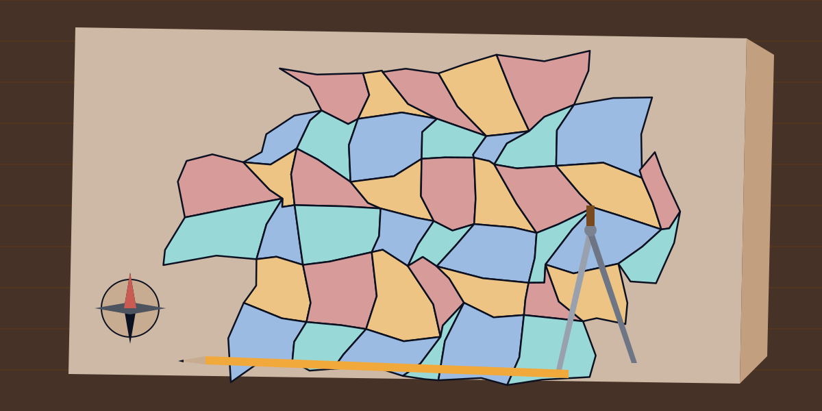
In 1852 Francis Guthrie, colouring a map of the counties of England, noticed that four colours seemed to be enough to keep any two counties that touched apart. Augustus De Morgan took up the question and it was in print by 1854. Alfred Kempe published a proof in 1879 and Peter Guthrie Tait another in 1880; Percy Heawood found the flaw in Kempe's in 1890, and proved in the same year that five colours always suffice. Four were shown to suffice in 1976, when Kenneth Appel and Wolfgang Haken announced a proof that reduced the question to 1,834 configurations (later 1,482) and handed them to a computer, which took over a thousand hours to check them. The proof was controversial at first because no person could check it by hand; Robertson, Sanders, Seymour and Thomas simplified it to 633 configurations in 1996, and in 2005 Georges Gonthier and Benjamin Werner had the Coq proof assistant check it in full.
The geography library for DKE, the Deterministic Knowledge Engine, writes some of a cartographer's work down in DKE Python, and this essay teaches the geography by reading it. You record three kinds of fact. A region is its name, the region it lies in directly and its level, and the library's rules conclude every region it lies within, to any depth. A map is the borders between regions and the colour each is given, and the rules conclude which regions are neighbours and which neighbours are given the same colour. A place is a latitude and a longitude, and a box a stretch of each, and the rules conclude which places lie in which boxes. Each answer names the facts it rests on, and correcting a fact withdraws the answers it supported. The second half of the library calculates: great circles on a sphere, geodesics on the ellipsoid, the Mercator projection and the area of a triangle on the Earth. Every program below runs as shown once the library's source file has been compiled into a store, and every output is copied from a run. Angles are in degrees and distances in metres.
1. Regions within regions
A country is divided into counties, and a county into municipalities, and a question about the country should find the municipality. The rules need only the parent each region names. A region lies within its parent, and within whatever its parent lies within:
@rule
def within_further():
    for r in Region, p in Region, q in Region:
        if Within.r.p == True and p.parent == q:
            Within.r.q = True
Here is Norway as it stood before 2020, with two counties, Hordaland and Sogn og Fjordane, and three municipalities. The rules also count what each region holds, at any depth:
import geography

geography.region("norway", "", "country")
geography.region("hordaland", "norway", "county")
geography.region("sogn_og_fjordane", "norway", "county")
geography.region("bergen", "hordaland", "municipality")
geography.region("askoy", "hordaland", "municipality")
geography.region("sogndal", "sogn_og_fjordane", "municipality")
print(geography.within("bergen"), geography.regions_in("norway", "municipality"))
holds = geography.Region("norway").holds
print(holds)
['hordaland', 'norway'] ['askoy', 'bergen', 'sogndal']
5Bergen lies within Hordaland and so within Norway, and Norway holds five regions. On 1 January 2020 the two counties were merged into Vestland, and Bergen, Askøy and Sogndal became its municipalities. Correct each municipality's parent, and the old answer goes with the fact it rested on. Then ask why Bergen is within Norway, and the answer is the chain of parents:
import geography

geography.region("vestland", "norway", "county")
for m in ["bergen", "askoy", "sogndal"]:
    geography.region(m, "vestland", "municipality")
print(geography.within("bergen"), geography.regions_in("vestland", "municipality"))
w = why(geography.Within.bergen.norway)
for c in w:
    print(str(c.path) + " = " + str(c.value))
['norway', 'vestland'] ['askoy', 'bergen', 'sogndal']
geography.Within.bergen.norway = True
geography.Within.bergen.vestland = True
geography.Region.bergen.parent = vestland
geography.Region.vestland.parent = norwayHordaland is no longer in the answer, because nothing says Bergen lies in it. Nothing was edited but the parents.
2. When two atlases disagree
Maps are made by people with views of the border. Hans Island, an islet in the Nares Strait between Canada's Ellesmere Island and Greenland, was claimed by both Canada and Denmark from 1973, when they settled their maritime boundary and left it out, until June 2022, when they agreed to divide it along a natural fault line. Each side's atlas put it in its own country, and a library that has to choose between the atlases would tell one of them it is wrong. This one reasons about both. It lets the two parents stand, unsettled() names what the sources disagree about, and no query refuses:
import geography

geography.region("canada", "", "country")
geography.region("denmark", "", "country")
geography.region("hans_island", "canada", "island")
update(geography.Region("hans_island").parent, "denmark", "a Danish map")
print(geography.unsettled())
print(geography.within("hans_island"))
print(geography.regions_in("canada", ""), geography.regions_in("denmark", ""))
['region hans_island parent']
['canada', 'denmark']
['hans_island'] ['hans_island']The island is within both countries, and each country holds it. Where the answer matters, the line that names the disputed fact is the one to read.
3. A map, and the colours it needs
The rules of a map are two. A border between two regions makes them neighbours both ways, and two neighbours given one colour clash. What a map needs of a cartographer is a colouring with no clash, and dsatur() chooses one by the method Daniel Brélaz published in 1979: colour next the region whose neighbours already show the most colours, the most neighbours breaking a tie and then the name, with the lowest colour none of them shows. It reads the borders and writes nothing, and paint() writes the colours it chose.
The map here is a wheel. Nevada borders Oregon, Idaho, Utah, Arizona and California, and those five border one another in a ring of five. A ring of an odd length cannot be coloured with two colours, and with Nevada in the middle it needs a colour of its own, so this map needs four:
import geography

for state in ["oregon", "idaho", "utah", "arizona", "california", "nevada"]:
    geography.region(state, "", "state")
for pair in [["nevada", "oregon"], ["nevada", "idaho"], ["nevada", "utah"], ["nevada", "arizona"], ["nevada", "california"], ["oregon", "idaho"], ["idaho", "utah"], ["utah", "arizona"], ["arizona", "california"], ["california", "oregon"]]:
    geography.border(pair[0], pair[1])
print(geography.neighbours("nevada"))
print(geography.dsatur())
geography.paint(["green", "yellow", "red", "blue"])
print(geography.clashes())
geography.colour("idaho", "green")
print(geography.clashes())
['arizona', 'california', 'idaho', 'oregon', 'utah']
{'nevada': 0, 'arizona': 1, 'california': 2, 'oregon': 1, 'idaho': 2, 'utah': 3}
[]
['idaho nevada']The numbers are the colours, counted from 0. Nevada has 0, and the ring of five needs three more, with Arizona and Oregon sharing one. paint() turned the numbers into a palette of four, and the map has no clash. Giving Idaho the colour of Nevada makes one, and clashes() names the pair.
dsatur() is a heuristic and not a proof. It is known to be exact for wheels, which is what this map is, and for bipartite graphs and cycles; in general it is not guaranteed to use the fewest colours a map allows, and the Four Colour Theorem says only that four always exist. Nothing in the library draws a map or checks that the borders written are the borders there are.
4. Places in boxes, and the line at 180
A box of latitude and longitude is the plainest region there is, and it has one awkward case. Longitude runs from -180 to 180 and a box that crosses the line where it wraps has a western edge east of its eastern one. The library reads such a box as the longitudes from the western edge round through 180 to the eastern, with two rules for the two halves:
if b.west > b.east and p.lat >= b.south and p.lat <= b.north and p.lon >= b.west:
    Inside.p.b = True
Kiribati's islands straddle the equator and the 180th meridian, which is why it has the most advanced time zone on Earth, UTC+14. A box that covers Tarawa, in the west, and Kiritimati, in the east, has a western edge at 169 degrees east and an eastern one at 150 west. A plain box with the same latitudes and a western edge east of 150 covers only Tarawa:
import geography

geography.place("tarawa", 1.45, 173.0)
geography.place("kiritimati", 1.87, -157.4)
geography.place("honolulu", 21.31, -157.86)
geography.place("auckland", -36.85, 174.76)
geography.place("suva", -18.14, 178.44)
geography.box("kiribati", -12.0, 5.0, 169.0, -150.0)
geography.box("plain", -12.0, 5.0, 150.0, 175.0)
print(geography.places_in("kiribati"))
print(geography.places_in("plain"))
['kiritimati', 'tarawa']
['tarawa']Honolulu at 21 degrees north, Auckland at 37 south and Suva at 18 south all lie outside the box's latitudes.
5. The great circle
The shortest path between two points on a sphere runs along a great circle, a circle whose centre is the sphere's. The distance along it is the central angle, the angle between the two points as seen from the centre, times the radius. The central angle the library finds by the haversine formula, which keeps its precision for points close together. The name is James Inman's, of 1835, a contraction of half-versed sine; tables of the function were printed from the first years of the century, because it saved a navigator multiplying and dividing by two. The radius is the Earth's mean, 6,371,008.8 metres.
The great circle from Oslo to Tokyo is the sort of path that surprises on a flat map. bearing() gives the course to set out on, destination() the point reached by keeping to the circle for a distance, and the bearing back is not the reverse of the bearing out:
import geography

d = geography.haversine(59.91, 10.75, 35.68, 139.69)
out = geography.bearing(59.91, 10.75, 35.68, 139.69)
back = geography.bearing(35.68, 139.69, 59.91, 10.75)
print(round(d / 1000, 1), round(out, 1), round(back, 1))
mid = geography.destination(59.91, 10.75, out, d / 2)
print(round(mid[0], 1), round(mid[1], 1))
end = geography.destination(59.91, 10.75, out, d)
print(round(end[0], 2), round(end[1], 2))
8406.3 40.7 336.3
66.4 101.6
35.68 139.69The distance is 8,406 kilometres. The bearing from Oslo is 40.7 degrees, north-east, and the bearing back from Tokyo is 336.3, which is not 220.7: a great circle crosses the meridians at an angle that keeps changing. The point half way is at 66.4 degrees north and 101.6 east, in northern Siberia, a little south of the Arctic Circle, which is at 66 degrees 34 minutes. The path from Oslo to Tokyo goes up before it comes down. Going the full distance on the same bearing reaches Tokyo, as it must.
6. The ellipsoid
The Earth is not a sphere but is flattened at the poles, and the sphere can be wrong by up to about half a per cent. The WGS84 ellipsoid has an equatorial radius of 6,378,137 metres and a flattening of 1/298.257223563. Thaddeus Vincenty published his iterations for the distance and azimuths between two points on an ellipsoid, and for the point a distance and an azimuth away, in Survey Review in April 1975, accurate to within half a millimetre on the ellipsoid. The library has both:
import geography

v = geography.vincenty_inverse(59.91, 10.75, 35.68, 139.69)
print(round(v[0] / 1000, 1), round(v[1], 1), round(v[2], 1), v[3])
print(round(geography.vincenty_inverse(0.0, 0.0, 1.0, 0.0)[0]), round(geography.vincenty_inverse(89.0, 0.0, 90.0, 0.0)[0]))
a = geography.destination(59.91, 10.75, 46.0, 1000000.0)
b = geography.vincenty_direct(59.91, 10.75, 46.0, 1000000.0)
print(round(a[0], 3), round(a[1], 3))
print(round(b[0], 3), round(b[1], 3))
print(geography.vincenty_inverse(0.0, 0.0, 0.5, 179.7))
8427.6 40.7 336.2 5.0
110574 111694
65.374 26.405
65.364 26.338
[0.0, 0.0, 0.0, -1.0]The ellipsoid says the same journey is 8,427.6 kilometres, not 8,406.3, a quarter of a per cent longer. A degree of latitude is 110,574 metres at the equator and 111,694 metres near the pole, which the figures in the second line reproduce, and a sphere cannot say that. Setting out from Oslo on a bearing of 46 degrees for a thousand kilometres, the sphere and the ellipsoid end about three kilometres apart.
The last line is the method's known limit. For points nearly opposite one another the iteration may fail to converge; after 200 rounds the library stops and returns zeros and a count of -1, where Vincenty's formulae in some other programs go on to return a wrong answer. In 2013 Charles Karney reformulated the inverse problem as a root-finding one that Newton's method solves quickly for every pair of points. The library keeps Vincenty's and says plainly where it fails.
7. Mercator
Gerardus Mercator published his map of the world in 1569 for sailors. It is cylindrical and conformal, so angles are kept, and a course of constant compass bearing, a rhumb line, is a straight line on it. Mercator did not explain how he built it, and the English mathematician Edward Wright published the first accurate tables in 1599. The northing is the natural logarithm of the tangent of 45 degrees plus half the latitude, in units of the Earth's radius, and the scale at a latitude is the secant:
return math.log(math.tan(math.pi / 4 + math.radians(lat) / 2))return 1 / math.cos(math.radians(lat))import geography
for lat in [30.0, 60.0, 70.0, 85.0]:
print(lat, round(geography.mercator(lat), 4), round(geography.mercator_scale(lat), 3))
y = geography.mercator(85.0511288)
print(round(y, 6), round(geography.mercator_inverse(y), 4))
d = geography.dms(59.91)
print(d[0], d[1], round(d[2], 2))30.0 0.5493 1.155
60.0 1.317 2.0
70.0 1.7354 2.924
85.0 3.1313 11.474
3.141593 85.0511
59.0 54.0 36.0At 60 degrees the scale is 2, so a short distance is drawn twice as long and an area four times as large, and at 85 degrees it is 11.5. This is why Greenland looks as big as Africa on the map, though Africa is about fourteen times its size. The 85.0511288 in the fifth line is the latitude at which the northing reaches the value pi, which is the half-width of the whole world's longitudes in the same units; the many online maps that use a Mercator cut off at plus and minus 85.05 degrees do so to keep the map square. mercator_inverse() returns the latitude, and dms() writes an angle as degrees, minutes and seconds.
8. A triangle on the Earth
On a plane the angles of a triangle add up to a half turn. On a sphere they add up to more, and the excess measured in radians, times the square of the radius, is the area, a theorem of Albert Girard's. L'Huilier's theorem finds the excess from the three sides alone, and the sides are great-circle distances the library already has. The first triangle has its corners at the point on the equator at 0 degrees, the one at 90 east and the north pole, and it is an eighth of the sphere. Its excess is half a pi, and its area is an eighth of the Earth's surface, which the last line checks against the whole sphere. The second is the Bermuda Triangle, whose corners Vincent Gaddis gave in 1964 as Miami, San Juan and Bermuda:
import geography
import math

print(geography.spherical_excess(0.0, 0.0, 0.0, 90.0, 90.0, 0.0))
octant = geography.triangle_area(0.0, 0.0, 0.0, 90.0, 90.0, 0.0)
print(round(octant / 1000000))
print(round(geography.triangle_area(25.76, -80.19, 32.30, -64.78, 18.47, -66.11) / 1000000))
r = geography.mean_radius()
print(round(4 * math.pi * r * r / 1000000))
1.5707963267948954
63758235
1144824
510065881An eighth of the Earth is 63.8 million square kilometres, and the whole is 510 million. The triangle between the three cities is 1.14 million square kilometres. Writers give the area as anything from 1.3 to 3.9 million, because each draws the corners where they please and no board names an official Bermuda Triangle. The library finds the area of a triangle with the corners it is given.
9. What the library leaves out
A region has one parent, so a country that is a member of an alliance, a river that is a border, or a territory two states hold is not a tree; the library reads the facts it is given. A border is a bare pair, so it cannot say how long the border is, where it runs, or that two regions meet at a point and not along a line, which matters to a colouring. dsatur() is a heuristic. The sphere has the mean radius and the ellipsoid is WGS84, and neither is the local datum a surveyor works in. Heights, the geoid, the Moon's pull on the sea and the changes of the plates are not there. The projection is Mercator alone. A box is a rectangle of latitudes and longitudes, not a country.
Closing
Guthrie coloured the counties of England and asked a question that took a hundred and twenty-four years and a computer to answer, and whose answer people still check. The library stays on the near side of that question. It says where a place is, in what, and which regions touch, writes down the colouring a method chooses and names the pair it finds clashing, and measures the Earth as the sphere and as the ellipsoid, with the difference between them in front of the reader. And because each conclusion names what it rests on, a reader who doubts one can ask why, and follow the answer down to the parent, the border or the coordinates it came from.